Bayesian Networks

Before reading this section, it may be helpful to visit my brief primer on graphs for an introduction to some of the terms used here.

Bayesian Networks

A Bayesian network (BN) is a graphical representation of a joint probability distribution, representing dependence and conditional independence relationships.

So what does this mean? Let’s go through the definition piece by piece.

graphical representation: A Bayesian network is drawn as a graph, with nodes and edges. In particular, BNs are DAGs, directed acyclic graphs, meaning that their edges have direction, and that there are no loops within the graph. In a functional network, the nodes represent the variables we are measuring and the edges represent interactions between them.
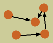
joint probability distribution: A joint probability distribution across a group of variables represents the probability of each of the variables taking on each of its values, given consideration of the values of the other variables. That is, it is not the collection of individual probabilities for each variable, but a joint distribution, allowing for the value of one variable to effect the value of another. For example, take two variables: sunshine and rain. While there may be a 60% probability of sunshine on any given day of the year, and a 25% probability of rain on any given day of the year, it is certainly reasonable to expect that whether or not there is sunshine on a particular day could interact with the probability of rain on that day. The joint probability distribution across sunshine and rain would take this into account.
dependence and conditional independence relationships: This concept is an extension of the above discussion. Two variables are dependent if knowledge of one provides predictive value for knowledge of another. For example, knowledge of the state of sunshine provides predictive value for the probability of rain.; Independence is the opposite, when knowledge of one variable provides no predictive value for the knowledge of another. For example, knowledge of the color of shirt you’re wearing provides no predictive value for the probability of rain.; Conditional independence comes into play when we have multiple variables that can all be correlated. For example, going back to our sunshine and rain variables, let’s add a third variable, whether or not you carry an umbrella with you. Let’s say you live in the moment, and only carry an umbrella if it is raining at the exact time you leave your house. In this case, while it is true that knowledge of sunshine provides predictive value for your umbrella carrying—because no sun means it is more likely to be raining, and thus more likely for you to be carrying an umbrella—this predictive value is entirely mediated through the variable of rain. If we already know whether or not it is raining, knowing whether or not it is sunny does not help further predict your umbrella carrying. Here, the two variables of your umbrella carrying and sunshine are conditionally independent given knowledge of rain.; This final concept of conditional independence is central to the power of Bayesian networks for functional network inference. It is what enables us to untangle the relationships among the variables within the network—whose values may all be correlated in some manner—and pick out direct influence.

All that is left now is to describe how the graphical representation indicates the dependence and conditional independence relationships in the joint probability distribution.

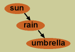
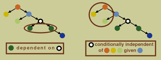
In a Bayesian network, dependence is indicated by directed edges. A child node is dependent on its parent node. For example, in the graph above, the dark green nodes are both dependent on the black and white node (see below). Additionally, any node is conditionally independent of its non-descendants, given its parent. For example, the black and white node is conditionally independent of the light green, orange, and yellow nodes, given the light blue node (its descends are the dark green and dark blue nodes, thus its non-descendants are all the other nodes; see below).

Dynamic Bayesian Networks

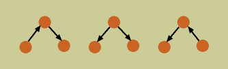
Bayesian networks do have some limitations for functional network inference. First, due to mathematical properties of the joint probability distribution, it is possible to have a group of BNs which represent exactly the same joint probability distribution, having the same conditional dependence and independence relationships, but which differ in the direction of some of their edges. Such a group is called an equivalence class of Bayesian networks (the BNs below represent an equivalence class). This creates problems in assigning direction of causation to an interaction from an edge in a Bayesian network.

Second, the restriction of the BN to be acyclic (also due to mathematical properities of the joint probability distribution) is a problem for biology, because feedback loops are a common biological feature. A BN could not model a feedback loop because it cannot have loops, or cycles.

Fortunately, both of these limitations can be overcome by using dynamic Bayesian networks (DBNs). A DBN consists of representing all variables at two (or more) points in time. Edges are drawn from the variables at the earlier time to those at the later time.

In this way, cycles over time can be represented using an underlying acyclic DBN. For example, in the DBN on the left above, we see that A at time t influences B at time t+1, B influences C, and C influences A. This represents a loop over time (on right), but the DBN has no loops. Additionally, there is no ambiguity over direction of edges—even if an equivalence class exists for this BN, we know the correct biological interpretation is that influence travels forward in time, not into the past!

Further Bayesian Network Resources

A good source to learn more about Bayesian networks, and Bayesian network inference algorithms, is B-Course, developed at the University of Helsinki. It also provides the opportunity to analyze your own data while learning.

Banjo is a Bayesian network inference algorithm developed by my collaborator, Alexander Hartemink at Duke University. It is the user-accessible successor to NetworkInference, the functional network inference algorithm we applied in the papers Smith et al. 2002 Bioinformatics 18:S216 and Smith et al. 2003 PSB 8:164.

And finally, here are some references which cover Bayesian networks in a more mathematically rigorous manner:

Friedman, N., Murphy, K. & Russell, S. 1998. Learning the structure of dynamic probabilistic networks. In Proc. Fourteenth Conf on Uncertainty in Artificial Intelligence, 139-147 (Morgan Kaufmann, San Francisco, CA).
Heckerman, D., Geiger, D. & Chickering, D.M. 1995. Learning Bayesian networks: The combination of knowledge and statistical data. Mach. Learn. 20, 197-243.